Dissecting the Dot Product | Math for Game Devs

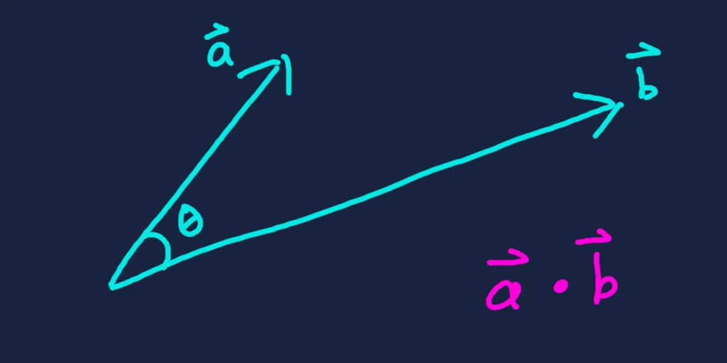
The dot product is a commonly used operation in game development. It has two equivalent definitions, shown below and labelled $(1)$ and $(2)$ for reference throughout this article. For any two vectors $\vec{a}$ and $\vec{b}$ with $n$ components, and the angle $\theta$ between them, their dot product $\vec{a} \cdot \vec{b}$ is defined as:

For example, take $\vec{a} = (3, 1)$ and $\vec{b} = (2, 3)$, where the angle between them is about $38.1^\circ$.

$$\begin{aligned} \vec{a}\cdot\vec{b} &= a_0 b_0 + a_1 b_1 \\ &= (3)(2) + (1)(3) \\ &= 9 \end{aligned}$$ $$\begin{aligned} \vec{a}\cdot\vec{b} &= \lVert\mathbf{a}\rVert\, \lVert\mathbf{b}\rVert \cos\theta \\ &= (\sqrt{10})\, (\sqrt{13})\, \cos(38.1^\circ) \\ &= 9 \end{aligned}$$

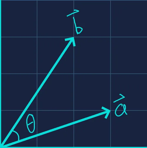
In most real-world code, we use equation $(1)$ since it doesn’t require knowing the angle $\theta$. But to better understand the geometry behind the dot product, let’s take a closer look at equation $(2)$.

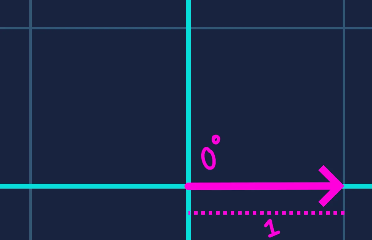
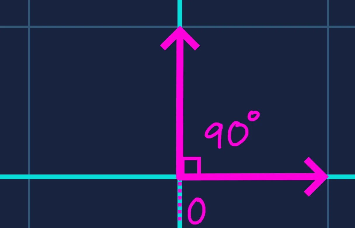
When $\vec{a}$ and $\vec{b}$ each have length 1 (that is, both are normalized), their dot product is simply $\cos\theta$:

$$\begin{aligned} \hat{a} \cdot \hat{b} &= \lVert\mathbf{a}\rVert\, \lVert\mathbf{b}\rVert \cos\theta \\ &= (1)(1) \cos\theta \\ &= \cos\theta \end{aligned}$$

Note that the notation $\hat{a}$ and $\hat{b}$ indicates that both are unit vectors of length 1.

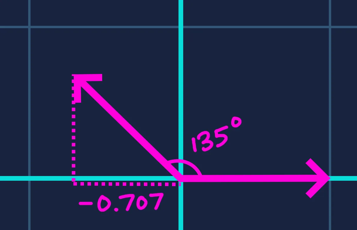
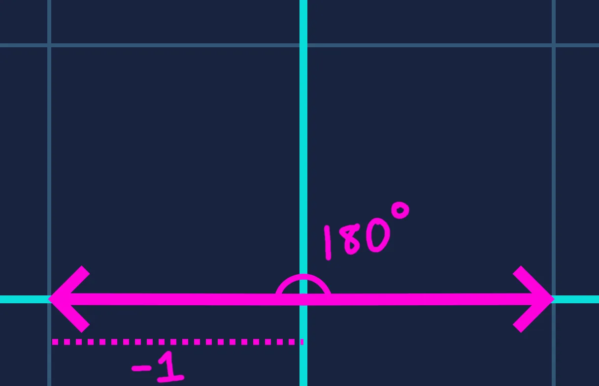
For any angle $\theta$, $\cos\theta$ always lies in the range $[-1, 1]$. This gives us a normalized measure of how aligned the two vectors are — the value directly reflects the angle between them.

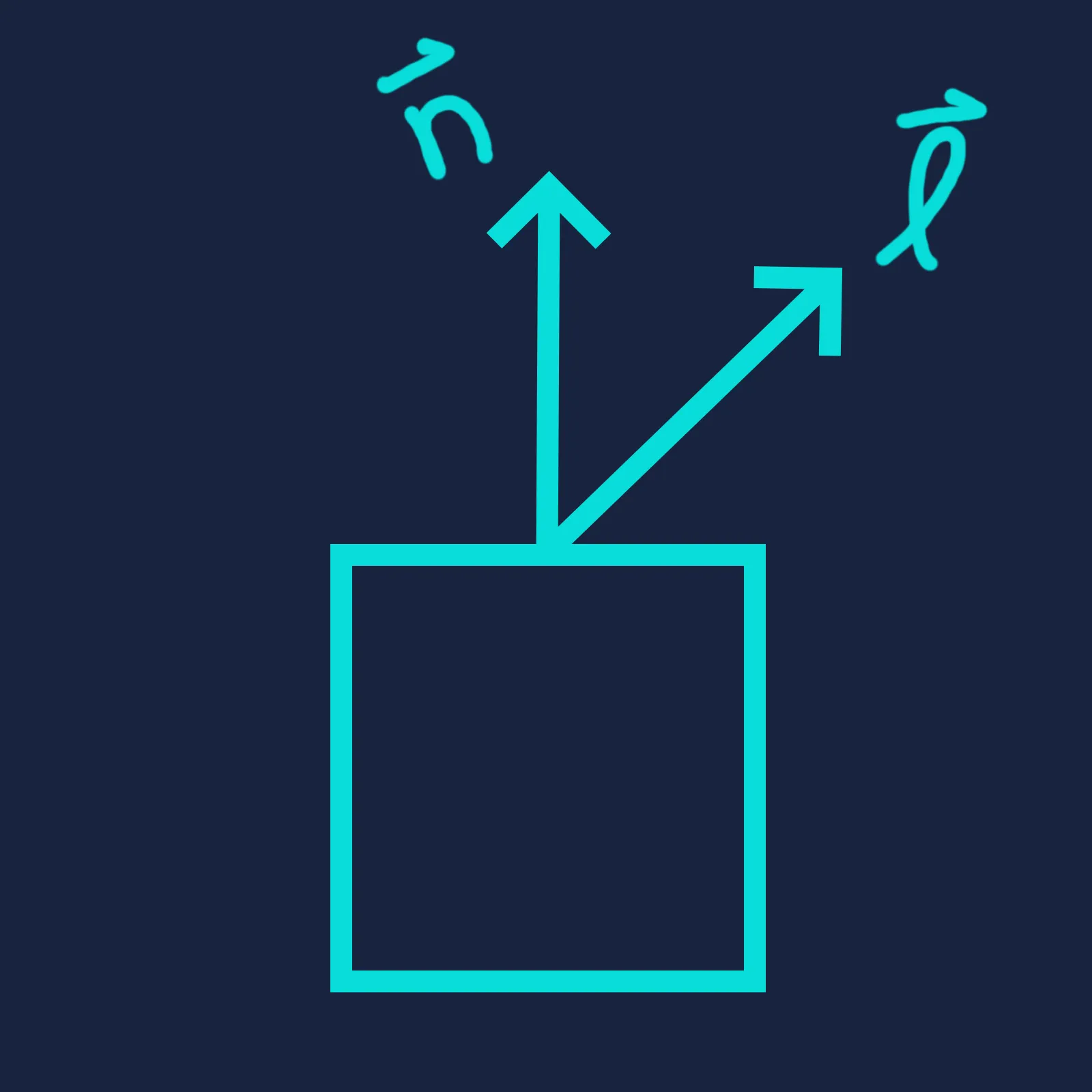
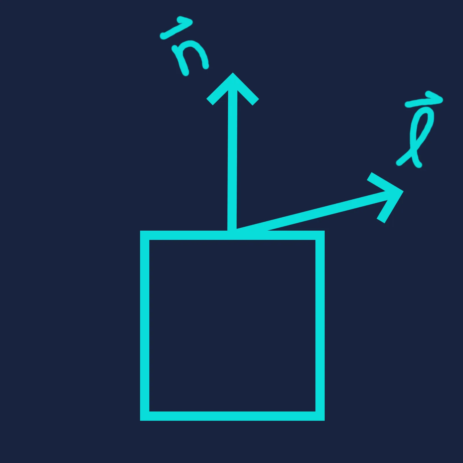
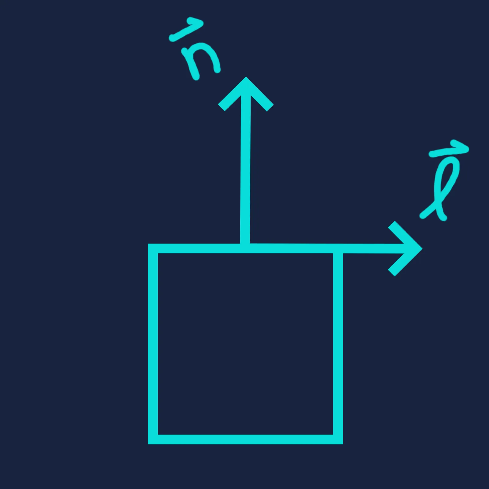
In graphics programming, this property is used to calculate the effects of directional lighting. The dot product between a surface’s normal vector (the direction perpendicular to the surface) and the direction toward a light source determines the brightness of that surface.

// GLSL shader

// Normalize the direction from the surface to the light
// such that the resulting dot product is in range [-1, 1].
// Assume that surfaceNormal is already normalized.
vec3 surfaceToLight = normalize(lightPos - surfacePos);
float brightness = dot(surfaceToLight, surfaceNormal);

// Clamp to [0, 1] - negative brightness does not make
// physical sense
float clampedBrightness = max(brightness, 0.0);

outputSurfaceColor = surfaceBaseColor * clampedBrightness;

As a result, the surface appears fully bright when the light is directly in front of it. The brightness drops off smoothly as the light moves around the surface, and fades to complete darkness when the light is to the side or behind.

It is hopefully intuitive that the dot product — and therefore the surface brightness — reaches its maximum when the light direction is fully aligned with the surface normal, and drops to zero when the two are perpendicular. But what can we say about the values in between?

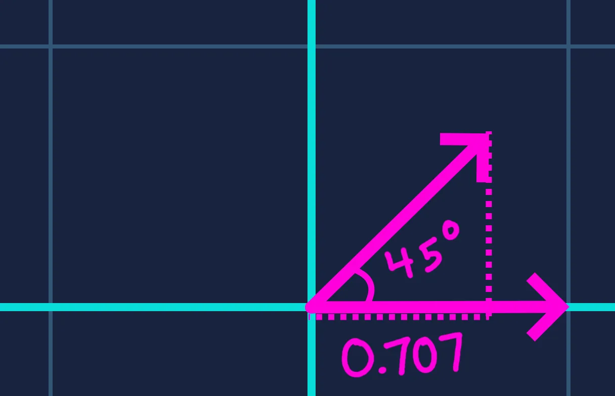
One thing we notice is that the cosine function is nonlinear with respect to $\theta$. The naive reasoning is that the surface would be at half brightness when the angle between its normal and the light direction is $45^\circ$. In reality, because cosine changes slowly near zero and faster at larger angles, the dot product only reaches $0.5$ when $\theta = 60^\circ$. In other words, brightness changes gradually when the light and surface are nearly aligned, but falls off much more rapidly as they diverge.

We can visualize this concept in terms of how much of the surface area is “visible” to the light. Redrawing the diagrams above from the light’s perspective, we see that half of the surface area faces the light when $\theta=60^\circ$. Therefore, the surface intercepts only half as much light energy as when the light is directly overhead, and consequently appears half as bright.

We can describe this changing rate of brightness more precisely using calculus. If you’ve taken a calculus class, you may recall that the derivative of $\cos\theta$ — its rate of change with respect to $\theta$ — is $-\sin\theta$. This explains why surface brightness decreases slowly when the surface normal and light direction are nearly aligned, but much more rapidly as they move apart.

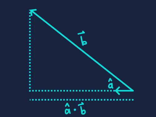
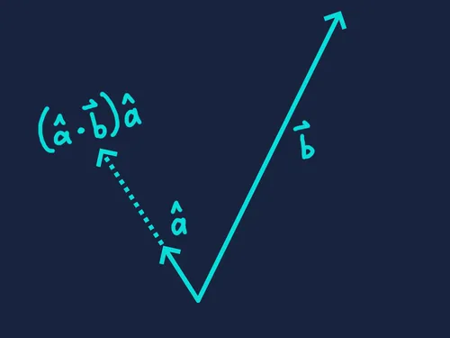
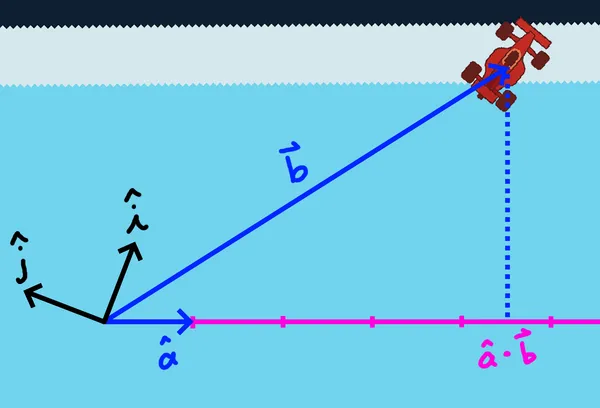
When $\vec{a}$ and $\vec{b}$ are both unit length, their dot product $\vec{a} \cdot \vec{b}$ measures how aligned they are — a value in the range $[-1, 1]$. Now let’s see what happens when only one of the vectors is normalized. We can interpret the dot product as the signed magnitude of the unnormalized vector’s component along the direction of the normalized vector.

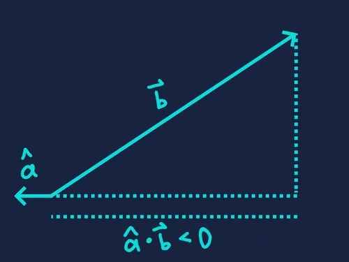
This value becomes negative when the unnormalized vector points in the opposite general direction — that is, when $\theta$ is greater than $90^\circ$ or less than $-90^\circ$.

The dot product itself gives a scalar. To get the corresponding 2D or 3D projection vector of $\vec{b}$ onto $\hat{a}$, multiply the dot product by the unit vector $\hat{a}$.

The dot product is commutative, meaning that $\vec{a} \cdot \vec{b}$ is always equal to $\vec{b} \cdot \vec{a}$. However, the result can differ depending on which vector is normalized. You can think of the normalized vector as defining a direction, and the other as the one being projected onto it.

This concept has a wide range of applications in game development. Let’s say we’re building a respawn system for a racing game. Players steer their vehicles along a looping track, and if they fall off, we want to respawn them at the closest point along the track’s centerline.

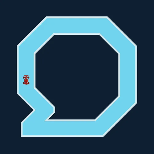
We can represent the track as an ordered list of position nodes, where each node connects to the next by a straight line segment along the track’s center. The final node connects back to the first, completing the loop.

// Rust
pub struct Track {
  pub nodes: Vec<Vec2>,
}

Let’s define a function to calculate the player’s respawn point.

pub fn calculate_respawn_point(
  player_pos: Vec2,
  track: &Track,
) -> Result<Vec2> {
  if track.nodes.len() < 3 {
      return Err(anyhow!("Incomplete track!"));
  }

  track.nodes.iter()
      .copied()
      .zip(track.nodes.iter().copied().cycle().skip(1))
      .map(|(curr_node, next_node)| {
          let track_dir = (next_node - curr_node).normalize();
          let rel_player_pos = player_pos - curr_node;
          let mut dist_along_track = rel_player_pos.dot(track_dir);

          let track_len = (next_node - curr_node).len();
          dist_along_track = dist_along_track.clamp(0.0, track_len);

          let closest_track_point = curr_node + dist_along_track * track_dir;
          let dist_from_track = (player_pos - closest_track_point).len();

          (dist_from_track, closest_track_point)
      }).min_by(|(a, _), (b, _)| a.total_cmp(b))
      .map(|(_, result)| Ok(result))
      .unwrap()
}

The function takes the position of the player when they left the track and returns where to place them back on the track after they respawn. It also takes the track data.

Breaking down the function, we first zip each track node with its succeeding node and iterate over each segment of the loop.

track.nodes.iter()
    .copied()
    .zip(track.nodes.iter().copied().cycle().skip(1))
    .map(|(curr_node, next_node)| {

Next, we compute how far along the current segment the player was when they left the track. This is the dot product of the player’s position relative to the segment start with the segment’s unit direction.

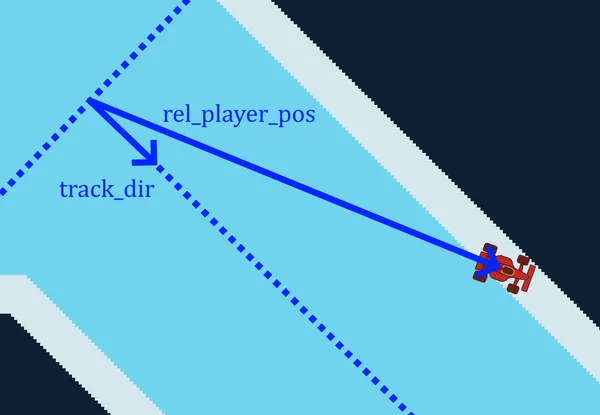
let track_dir = (next_node - curr_node).normalize();
let rel_player_pos = player_pos - curr_node;
let mut dist_along_track = rel_player_pos.dot(track_dir);

We clamp the player’s position along the current segment so it stays within the segment’s endpoints.

let track_len = (next_node - curr_node).len();
dist_along_track = dist_along_track.clamp(0.0, track_len);

Finally, we project onto the segment to get a candidate respawn point, then return the candidate with the smallest distance to the player’s position.

  let closest_track_point = curr_node + dist_along_track * track_dir;
  let dist_from_track = (player_pos - closest_track_point).len();

  (dist_from_track, closest_track_point)
}).min_by(|(a, _), (b, _)| a.total_cmp(b))
.map(|(_, result)| Ok(result))
.unwrap()

Now, when the player falls off, they’re respawned at the closest point along the centerline of the track!

We’ve explored cases where at least one vector in the dot product has unit length — but what about when neither vector is normalized? We’ll come back to that question in a bit.

Up to this point, we haven’t really discussed equation $(1)$ — only noted that it’s often used in practice to compute the dot product when the angle $\theta$ between vectors isn’t known. At first glance, equations $(1)$ and $(2)$ look nothing alike — so how can they produce the same result?

Suppose we’re taking the dot product of two vectors $\hat{a}=(0.8, 0.6)$ and $\vec{b}=(2, 4)$. Notice that $\hat{a}$ has unit length. We can write out the dot product as follows.

$$\hat{a} \cdot \vec{b} = \begin{bmatrix} 0.8 \\ 0.6 \end{bmatrix} \cdot \begin{bmatrix} 2 \\ 4 \end{bmatrix} = 4$$

Now let’s turn $\hat{a}$ on its side.

$$A \vec{b} = \begin{bmatrix} 0.8 & 0.6 \end{bmatrix} \begin{bmatrix} 2 \\ 4 \end{bmatrix} = 4$$

We’ve now expressed the dot product as a matrix–vector multiplication that produces the same scalar result. Matrix $A$ is applying some linear transformation to $\vec{b}$. If you’re familiar with transformation matrices typically used in game development — such as world matrices, view matrices, and projection matrices — ${A}$ might look unusual (if you’re not familiar, I’d recommend reading up on them!). Typical transformation matrices are $2\times2$, $3\times3$, or $4\times4$, mapping a vector to another vector of the same dimension. By contrast, $A$ is $2\times1$, mapping a 2D vector to a single scalar value.

This transformation essentially says, “give me $0.8$ for every unit of $\vec{b}\,$‘s first component, and $0.6$ for every unit of its second component”. We can visualize this by imagining a number line defined by $\hat{a}$ — the one-dimensional space onto which $\vec{b}$ is projected.

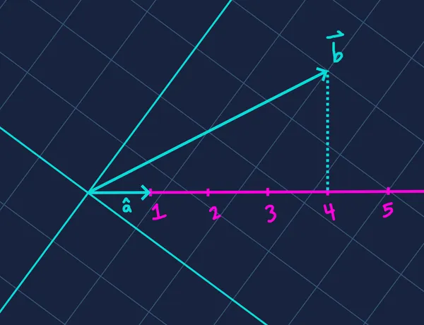
The projected value along $\hat{a}$ increases linearly with each component of $\vec{b}$. A change in $b_0$ (the x component) always affects the result by the same amount, regardless of $b_1$ (the y component) — and vice versa. Each component contributes independently to the final value.

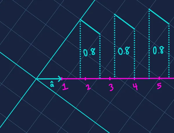
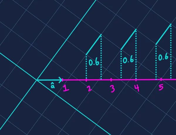
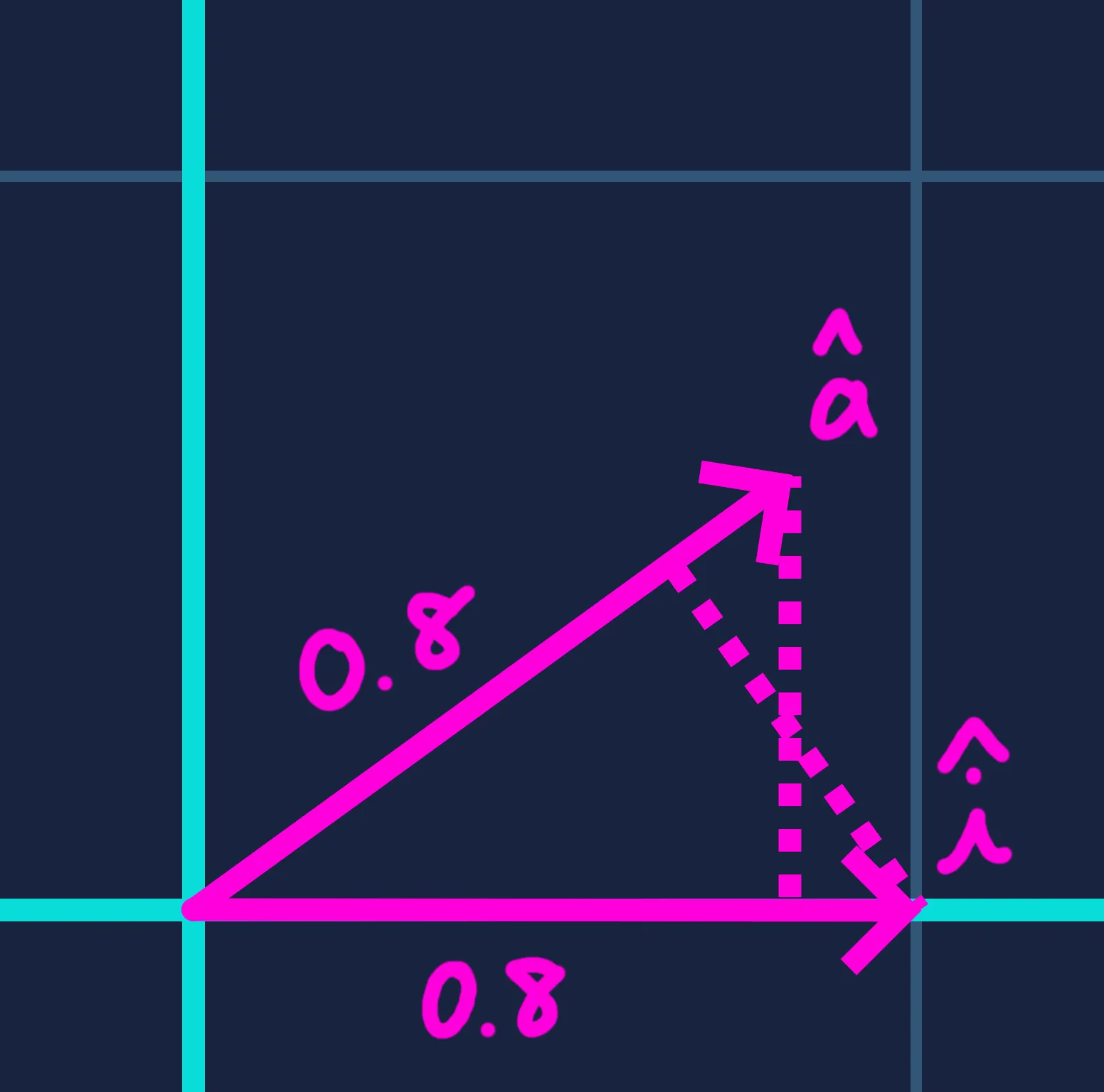
Visualizing $\hat{a}$ as a one-dimensional number line is key to understanding the dot product’s projective nature. But how do we know for sure that each unit of $b_0$ contributes exactly $0.8$ to the result, and each unit of $b_1$ contributes exactly $0.6$?

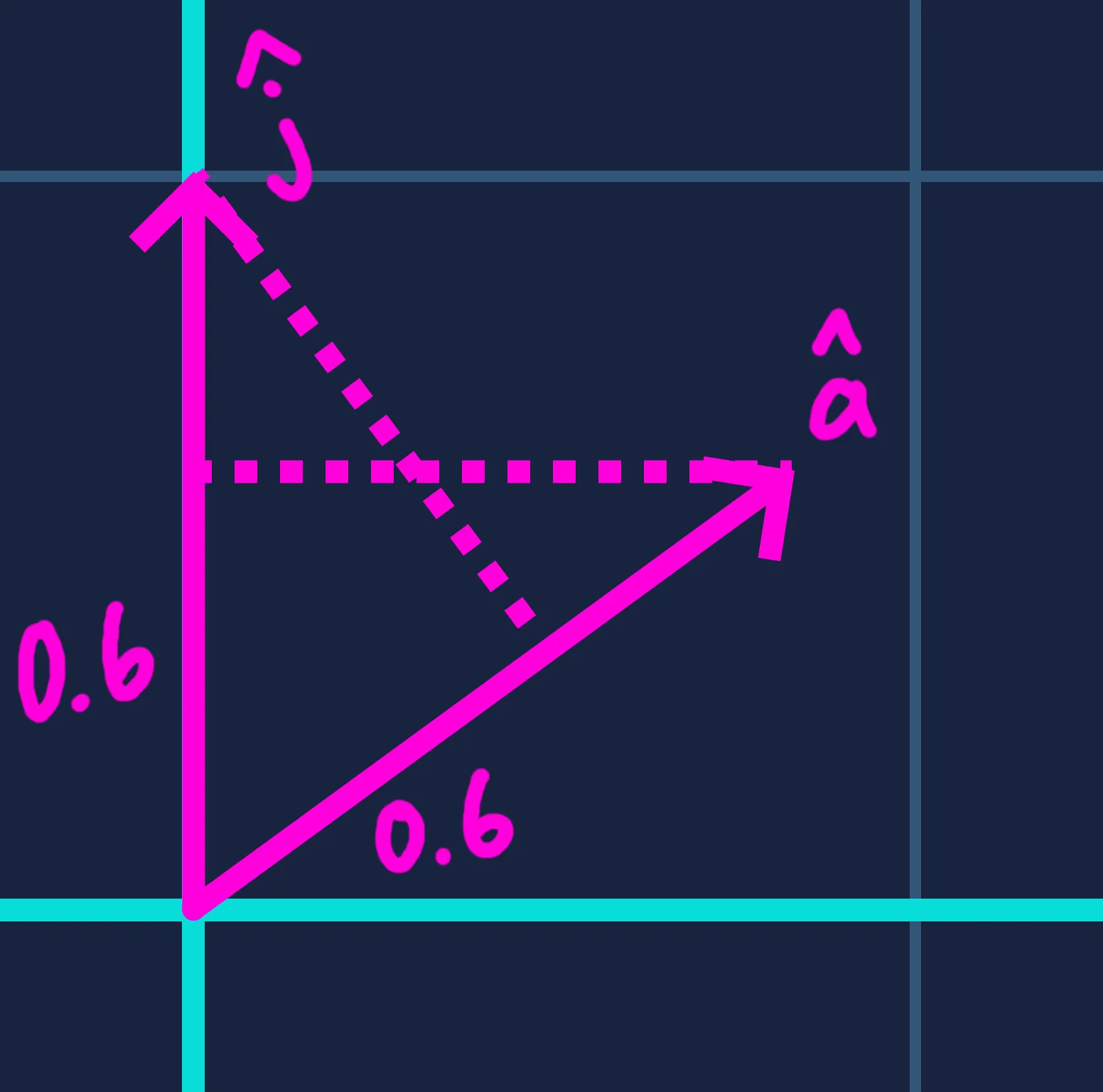
Let $\hat{i}$ be the unit vector along $b_0$‘s axis (the x-axis). Since $\hat{a}$ projects to $0.8$ on the $\hat{i}$ axis, and both $\hat{a}$ and $\hat{i}$ have unit length, we can argue — by symmetry — that $\hat{i}$ projects to $0.8$ along $\hat{a}\,$‘s axis as well. A similar argument holds for $a_1$, $b_1$, and $\hat{j}$, the y-axis.

In other words, every unit of $b_0$ adds $0.8$ to the projection onto $\hat{a}$, and every unit of $b_1$ adds $0.6$.

When $\hat{a}$ has unit length, it preserves the scale of the space in which $\vec{b}$ resides. For example, if $b_0$ and $b_1$ are in meters, then $\hat{a} \cdot \vec{b}$ is also in meters. If $\vec{a}$ instead has length 9, then $\vec{a} \cdot \vec{b}$ transforms $\vec{b}$ into a one-dimensional space where each unit of $\vec{b}$ contributes nine times as much — or is “worth” nine times as much — as when $\vec{a}$ is normalized. This case has less geometric meaning, which is why in most game scenarios, at least one vector is normalized before taking the dot product. There are, however, situations where the magnitudes of both vectors carry real meaning. For instance, in physics, work — the energy transferred to or from an object — is computed as the dot product of a force vector and a displacement vector.

We can see this linear transformation in effect with an overlay on our racing game example. Take a moment to digest it all.

The dot product appears in countless ways throughout game development. With this understanding, you’re now better equipped to recognize its role when studying new algorithms or designing interactions in your own projects.

Thank you for reading!

Key points:

• The dot product of two vectors has two equivalent definitions: $(1)$ and $(2)$.
• When both $\hat{a}$ and $\hat{b}$ are unit vectors, $\hat{a} \cdot \hat{b}$ lies in the range $[-1, 1]$ and represents how aligned the two directions are.
• When $\hat{a}$ is unit length, $\hat{a} \cdot \vec{b}$ gives the scalar distance covered by $\vec{b}$ along $\hat{a}\,$‘s direction. The projection of $\vec{b}$ onto $\hat{a}$ — the point on $\hat{a}\,$‘s axis closest to $\vec{b}$ — is obtained by multiplying that scalar by $\hat{a}$.
• More generally, $\vec{a} \cdot \vec{b}$ can be viewed as a matrix–vector product $A\vec{b}$, where $A$ (a $1 \times n$ row matrix) linearly transforms $\vec{b}$ onto the one-dimensional number line defined by $\vec{a}$.

— TheHurtDev